Running an Optimal Trace
The goal of tracing (historically called redlining) is to complete all of the trails in a given area. This game originates from the New Hampshire hiking community, where a White Mountains trace involves covering over 1,450 miles of unique trails.
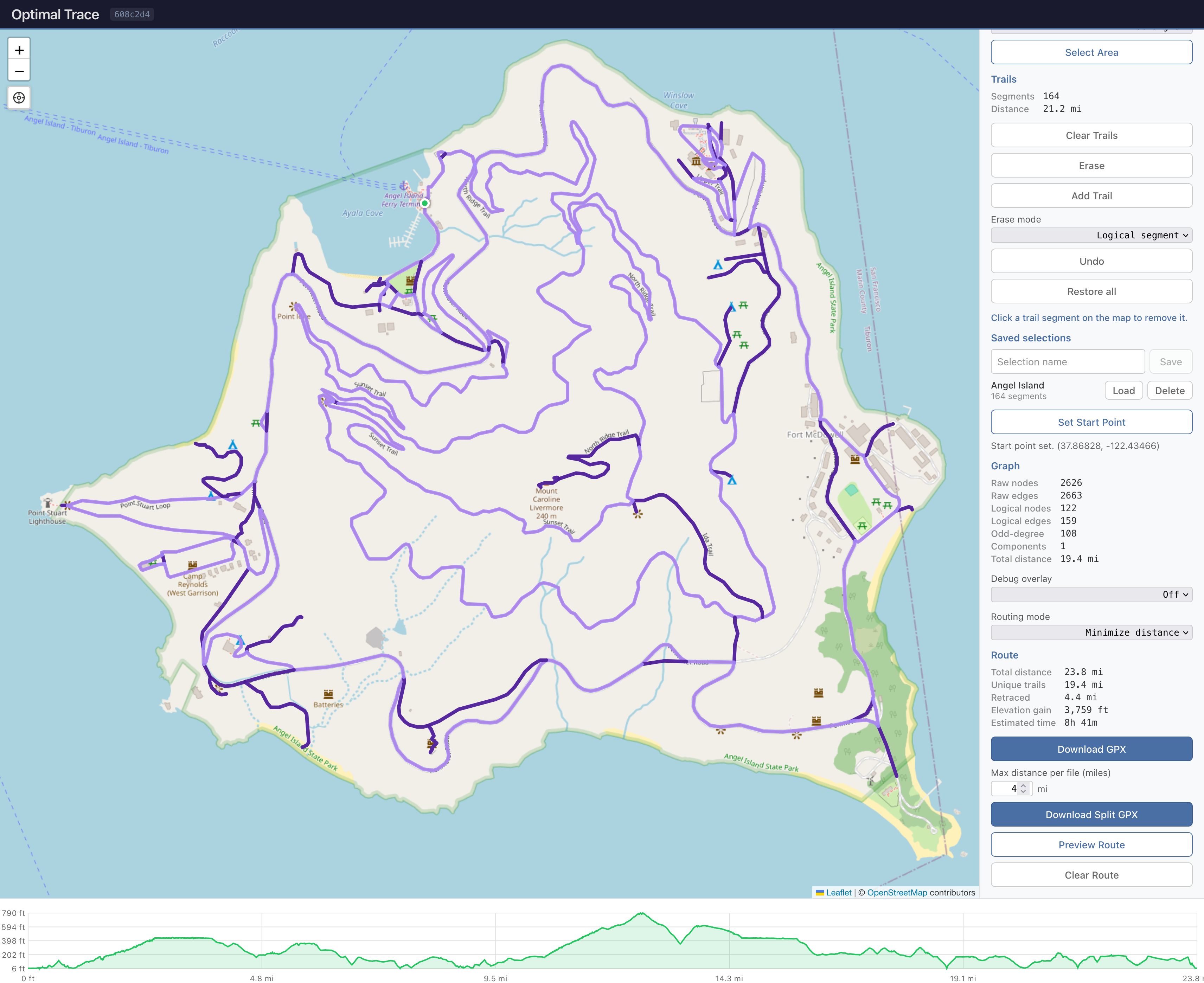
Inspired by a friend’s long run in the state park, I wanted to trace San Francisco’s Angel Island in a single run. I struggled to manually plan an efficient route covering the island’s dense network of 19.4 miles of unique road/trail. Hoping to avoid an ultramarathon, I wrote some software for planning and executing optimal traces.
Optimal trace of Angel Island. Red: included trails. Light purple: unique segments. Dark purple: repeated segments.
Before Angel Island, I did three local test runs, on Mount Sutro (Strava, JPG), Mount Davidson (Strava, JPG), and Glen Canyon (Strava, JPG).
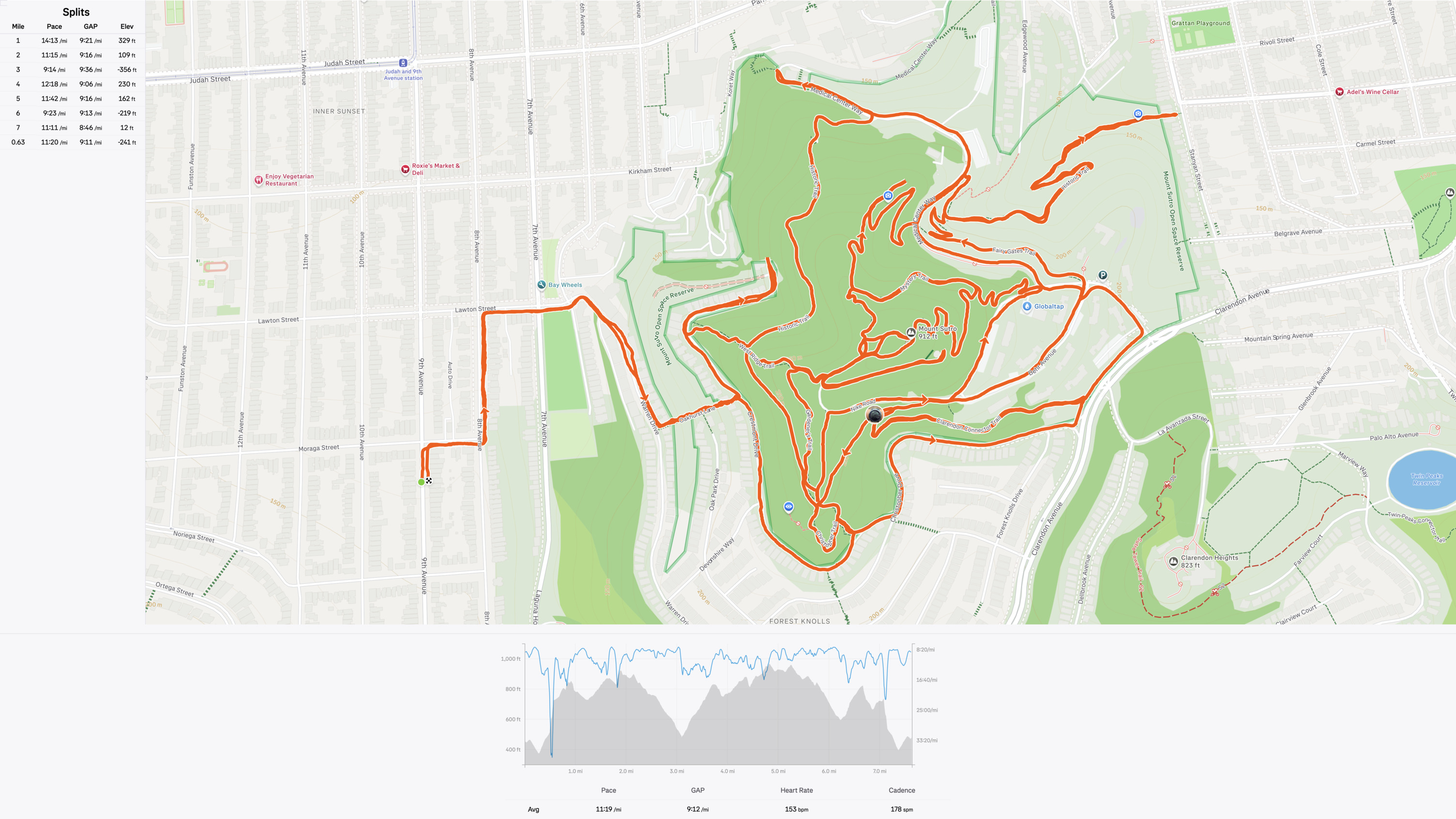
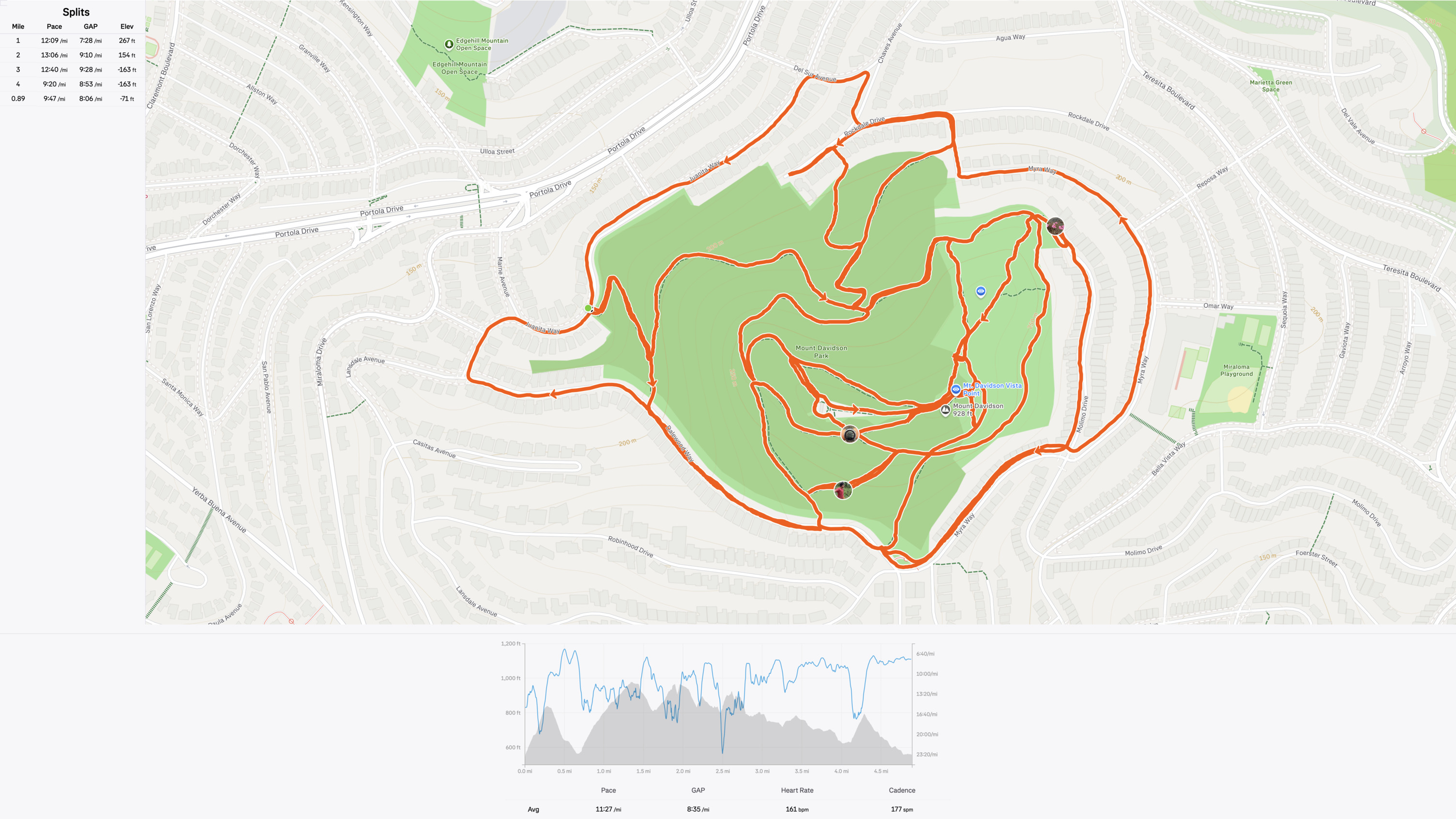
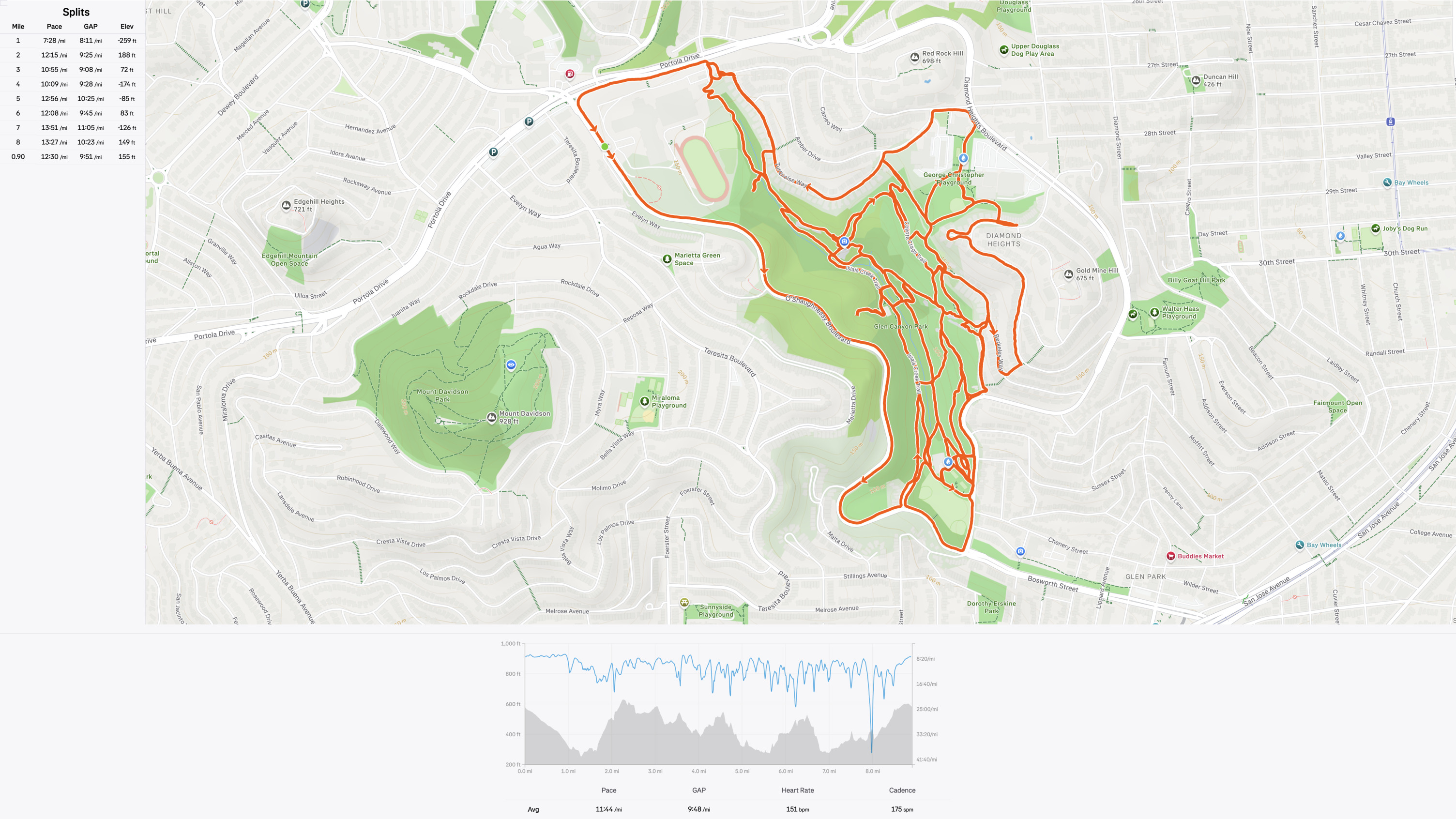
Over those test runs, I refined: the technique for scouting the location, using maps such as popularity heat maps and satellite maps to determine which trails to include; the tooling for selecting the trails in the web app I built, fetching trail data from an API and having an interface for manually adding/removing trails; the algorithms for optimizing the route, implementing a solver for the Chinese postman problem; and the process for following the course, using a combination of live navigation on my watch and maps on my phone.
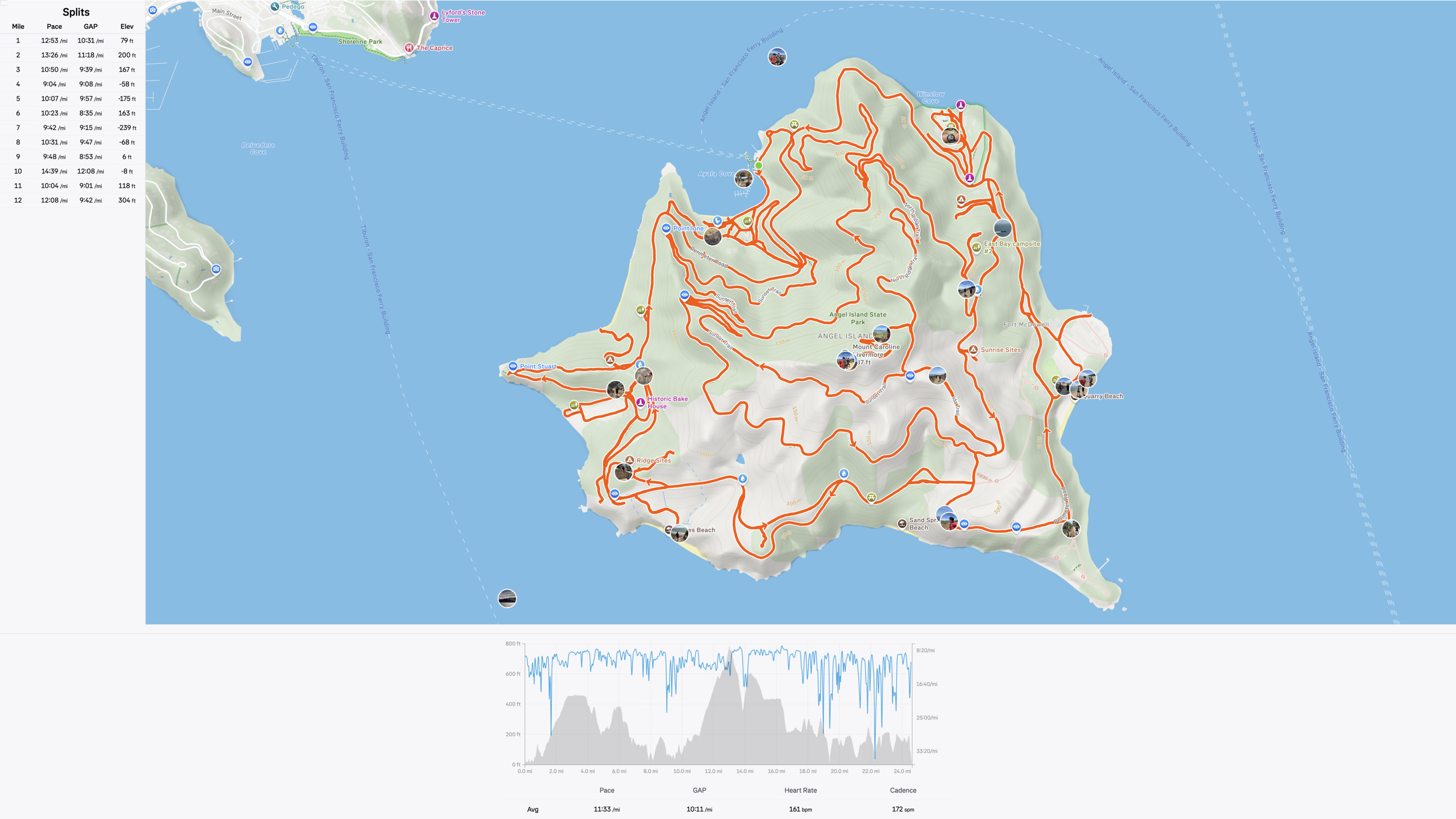
For the Angel Island run (planned route, Strava, JPG), I optimized for minimizing total distance; the planned route ended up being 23.8 miles in total, including 4.4 miles of retraced trails. Our actual distance was 24.6 miles, including some detours, which we finished in about five hours.
Scouting the location
The first step of planning an optimal trace is deciding which trails to include. For it to be a trace, it is necessary to include all of the trails in the chosen area. But it is critical to avoid nonexistent or impassable trails. Because the route has to be planned and optimized ahead of time, discovering partway through a run that a segment cannot be traversed would break the route. It is not always possible to adjust the route on-the-fly in such situations without breaking optimality.
OpenStreetMap
As a baseline, I was using OpenStreetMap to identify the roads and trails in a given area. This is the main map database used by Strava, for example.
Popularity heat maps
Services like Strava and Garmin Connect offer popularity heat maps that are helpful for identifying closed or nonexistent trails. For example, the heat map provides strong evidence that the Sunset Trail on Mount Sutro is closed.

Working with the heat map poses a couple challenges. It aggregates activities over a long time horizon, so it does not capture recently closed trails. The algorithm does some clipping and normalization, so it does not show very unpopular trails. To some degree, this can be overcome by using sport-specific heat maps. For example, comparing the all-sports heat map with the hiking-specific heat map on Mount Davidson reveals a couple additional trails that do get some traffic.

Satellite maps
For my test run on Mount Davidson, I omitted one trail that was not highlighted on the heat map, but during the run, I found that it was indeed a real trail. Later, I realized that I could have identified this by looking at the satellite map.

Street view
When there is recent street view data available, it can be a good way to confirm trail closures or inaccessible areas. For example, the Sutro Sunset Trail closure can be confirmed this way.

Park maps
Official maps provide the clearest guidance on inaccessible areas. For example, the Angel Island park map depicts service roads and Coast Guard areas that are off-limits to visitors, despite them appearing on the Strava heat map.

For the Angel Island run, I spent a couple hours scouting the area using all of the above methods. Despite my best efforts, I made small errors in both directions while planning: the route was missing an out-and-back to Battery Ledyard in the southwest part of the island, which we saw and added on the run; and the route had a phantom trail on the northwest part of the island where Perimeter Road connects to Sunset Trail, which we dropped on the run after it became apparent that it was not a real trail. Thankfully, these errors did not end up having an impact on the optimality of the route.
Selecting the trails
I used the Overpass API to retrieve all the roads and trails in a given area. The API offers some basic filtering capabilities, but all my runs required making manual edits to the retrieved data.
Deleting edges
The retrieved data had segments that were impassable, as determined by scouting, or had noise such as connectors to buildings, offshoots for bus stops, or sidewalks included separately from roads. I needed to delete these before path optimization.
The raw data from OpenStreetMap consists of a graph with thousands of nodes, even for small areas. To make for a good editing experience, I built an interface that supports working with either physical nodes and edges corresponding to the original data from OpenStreetMap or logical nodes that include only trail junctions and logical edges that group together all physical edges between junctions.
Adding edges
This was a rare occurrence, but the OpenStreetMap data was occasionally missing paths whose existence could be confirmed via other means such as satellite maps. For this reason, I needed to be able to add edges to the map.
Optimizing the route
Initially, I only considered optimizing for distance. After a hilly run on Mount Davidson, I thought about minimizing elevation or estimated travel time. For elevation, I used the USGS 3DEP API to fetch fine-grained elevation data; initially, my software wildly overestimated elevation gain, which was fixed by requiring a minimum threshold (of 2 meters) to count elevation changes. For estimating travel time, I used Tobler’s hiking function to compute grade-adjusted pace; this calculation used a moving average to smooth the elevation profile.
The distance and elevation optimization objectives correspond to a well-known combinatorial optimization problem called the Chinese postman problem, which is to find a circuit that minimizes the sum of edge weights and covers every edge in a graph. Luckily, this problem has a practically efficient polynomial-time solution. As an additional optimization, I computed the optimal path over the logical graph, where the logical edge weights were the sums of the corresponding physical edge weights, and then mapped the solution back to the physical graph.
I found that the distance and elevation optimization objectives yielded similar solutions. For example, on Mount Davidson:
| Optimization Objective | Distance | Elevation |
|---|---|---|
| Distance | 5.0 mi | 1,410 ft |
| Elevation | 5.4 mi | 1,273 ft |
Unsurprisingly, optimizing for elevation repeats some longer and flatter road segments, while optimizing for distance repeats some shorter and steeper trail segments.
Optimal traces of Mount Davidson with different optimization objectives. Light purple: unique segments. Dark purple: repeated segments.
Optimizing for time is slightly different: in this setting, the cost to traverse an edge depends on the direction in which the edge is traversed, because it takes longer to run uphill than it takes to run downhill. This problem is known as the windy postman problem, and it is NP-hard. The solution I used, based on integer linear programming, worked only for small graphs, so I did not use it in practice.
On my runs, the elevation savings did not seem worth the added distance, so I always opted to minimize distance.
Following the course
It took several iterations to develop a good process for following a route while on a run. My original plan was to export a GPX of an optimal trace, import it into Strava, and follow the route using my phone. The final process ended up being considerably more involved.
3D GPX
The first iteration of the software exported a flat GPX, with no elevation data.
<trkpt lat="37.7579435" lon="-122.4597985"></trkpt>
<trkpt lat="37.7578609" lon="-122.4598050"></trkpt>
<trkpt lat="37.7577141" lon="-122.4597455"></trkpt>
Importing this into Strava would fill in the elevation data. Unfortunately, the import process was buggy, apparently misplacing or omitting certain nodes.

Opening the original GPX in other software displayed the correct path, but some software did not support previewing the route without elevation data. These errors were fixed once I added elevation to the GPX export itself, originally relying on the Open-Meteo elevation API, which provides GLO-90 data with 90-meter resolution. Later, I switched to the USGS 3DEP API, which dynamically provides the best available data, up to S1M with a 1-meter resolution.
<trkpt lat="37.7579435" lon="-122.4597985">
  <ele>238.2</ele>
</trkpt>
<trkpt lat="37.7578609" lon="-122.4598050">
  <ele>239.1</ele>
</trkpt>
<trkpt lat="37.7577141" lon="-122.4597455">
  <ele>239.2</ele>
</trkpt>
This fixed the Strava import as well as compatibility with other software.

Garmin navigation
Repeated segments were impossible to see on a static Strava route on my phone, so I also synced the route to my Garmin watch for live navigation while running. This was helpful, but an imperfect solution in dense areas.

Navigation on a 1.3” 260x260px memory-in-pixel display.
Strava route preview
On my first test run on Sutro, I had the static Strava maps plus Garmin navigation, but I got confused as soon as I got to an area with dense trails. After a brief pause, I came up with the idea to use Strava’s route preview feature to animate the route, where I could also scrub to look carefully through particular parts of the route. While this is not the intended use case of the feature, it got me through the first test run.
Organic Maps
Strava’s route preview feature is designed for aesthetic purposes rather than as a navigation tool. It only supports a satellite map as the base map, does not handle overlapping segments well, and does not show your current location. For my second test run, I switched to using Organic Maps to visualize the GPX exported by my software.
This setup had several advantages: showing the current location on the map, better resolution on scrubbing, and supporting tapping a point on the map to find it on the planned route.
Split GPX
My longest test run before Angel Island was 8.5 miles. While preparing for the 24-mile Angel Island run, I found that the resolution when scrubbing was inadequate for navigating dense areas.
I worked around this by implementing a split GPX export, where the path was chunked into 4-mile segments. This provided adequate resolution when scrubbing through the segment. Color-coding the segments and being able to show/hide them independently in Organic Maps also simplified navigation.
Using the combination of live navigation on my Garmin watch and Organic Maps on my phone, I was able to navigate successfully over the course of the Angel Island run.
Try it yourself
The optimal trace planning software runs entirely client-side in the web browser and uses public APIs that do not require authentication. You can try the app at optimal-trace.anish.io. Note, the web app is not mobile-optimized.
Source code is available at github.com/anishathalye/optimal-trace.